Basic Neural Network

For building a simple neural network, we decided to leverage Pytorch and Google Colab. We developed our initial networks in Colab, and switched over to developing our networks locally once we transitioned to testing our networks in our Gazebo-ROS simulation.

Basic Neural Network

Initial Development

To make sure we could build a functional neural network in pytorch, we decided to start off with a simple network. This one has an input size of 3, which is just the x position, y position, and y velocity of a ball. The x and y positions would come in as being relative to the robot’s position, and the ball only has a velocity component along the y axis. The output size of the network is 1, which is the x velocity to move the robot. We used a mean square error loss function and no intermediate layers or activation functions. We specifically chose to use a mean square error loss function because we wanted the output of our model to be continuous, and mean square error loss functions are useful for continuous outputs.

To get data for testing this, we created a small simulation with the robot moving along the x axis, and one ball coming towards it along the y axis. For our simulation, we could input initial conditions for the ball: x position relative to the robot, y position relative to the robot, and velocity along the y-axis. Then, the simulation would run its main loop where if the ball’s y-axis was in line with the robot, the robot would simply set its velocity so that it would move out of the way. The simulation would terminate either when the ball went past the robot, or when it hit some prespecified max number of steps to prevent overly long calculations. Each step of the simulation generated a data point which captured the ball’s state and the robot’s velocity at that step as a row in a numpy matrix. We ran this simulation for a variety of initial conditions for the ball’s state and recorded the results. This was the data that we then used for testing our neural network.

Since our network was only a single layer with no activation functions, we could expect it to behave like linear regression. By comparing this network we’ve trained in pytorch to a linear regression model from numpy, we were able to check whether or not we created our pytorch model properly and if it was acting as expected. To do this, we compared the mean square error of the pytorch neural network model to the numpy linear regression model after they had each been fit. Since the errors matched, it meant that they were each creating the same model, and that we were properly using Pytorch.

We decided to leave this network soon after we created it as we realized that the function we wanted our network to learn was inherently nonlinear, even through the data it collected from our basic simulation. Remember, our goal is for the network to learn a function that maps ball state(s) to a robot velocity. In our basic simulation for training data, our robot would only move when a ball’s x position relative to the robot was approximately 0. At all other times, we the robot would do nothing as it wasn’t in danger of being hit by a ball. If we plotted the desired function from the ball’s relative x position to the robot’s velocity, it would look like a flat line until the relative x position was exactly 0, at which point the velocity would spike up or down depending on which way the robot needed to move, and then go back to being a flat line shortly after. This function cannot be approximated well enough for our purposes with only a linear mapping.

Second Pass:

Once we knew we could successfully create a neural network and train it using Pytorch, we began working on our first implementation that would be compatible with our simulation in Gazebo, which rolled multiple balls towards the robot at varying angles and velocities.

Our input for this model was quite different. We wanted to experiment with data pre-processing and we were curious how our model would work with several balls as inputs. One of the unique challenges of working with the ball states was that we wanted the ball states to be in some kind of order when we put them into the network. More specifically, we decided to order them by proximity to the ball. This decision was made with the intent that the network would put heavier weights on the state for the ball that was closest to it, and the closest ball would always be represented by the same inputs. In terms of data preprocessing, we decided to represent each ball with 3 inputs: distance from the robot, speed, and angle of attack. The angle of attack represents the difference between heading of the ball and the angle from the robot to the ball (i.e. an angle of 0 means the ball is projected to hit the robot, and an angle of +10 degrees means that the ball is projected to pass to the front of the robot). Our hope was that this information would be everything the robot needed to dodge balls. Since we were inputting 2 ball states into our network, and each ball state was composed of 3 inputs, we were inputting a total of 6 inputs into our network.

We decided to add an intermediate layer and an activation function to use between every layer to add some abstraction and nonlinearity to our model. We added a single intermediate layer of size 4 so the intermediate layer would be condensing the data from the first layer, and also abstracting out some abstract representation about the ball states. This abstraction is necessary for more complex, nonlinear functions. The thing we needed to balance here was that if we added too many layers or made our model too big, then our network would take a longer time to train without necessarily producing better results. This is because more layers mean more weights for the network to learn.

We also realized that it could be potentially quite useful to be able to be able to specifically try out specific cases more granularly than we could with the Gazebo simulation. To this end, we built a visualizer with a simple GUI that allowed us to specify two ball states with a visual representation of what those ball states would actually look like and a visualization of what the network output as a robot velocity. In addition to this, we added a simple plot utility that would show us the loss of the network over time. This made it possible for us to quickly check whether the network was actually learning anything, and whether it was overfitting to our training data.

This is what our gui looked like in Google Colab. 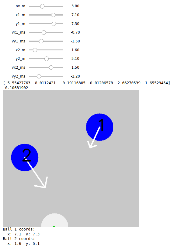All we had to do was move the sliders for the different ball positions, velocities, and robot positions, and then we would see a green arrow at the bottom that indicated where the robot was going to move in response to those inputs and how fast.

To implement this in Gazebo, we added an option to our main processing node to load in a pytorch model and use it to drive the robot. We also decided to port over the model training, the visualizer, and the plotting functionality into local Python scripts rather than separating them into Google Colab notebooks to make our workflow smoother.

This is what the gui looked like when run locally. 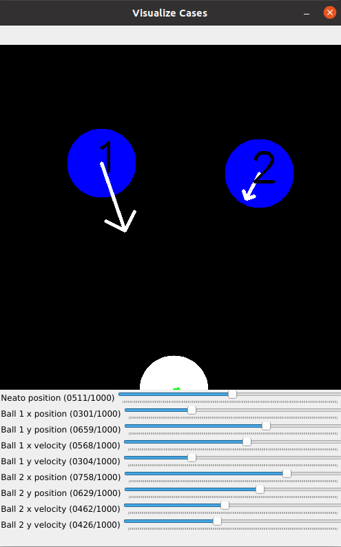If you look at the values set by the sliders, you’ll notice that they aren’t nice floating point numbers. This is because we wanted an easy way to port the visualizer into a local script with minimal refactoring, and the best way we found to do this was through a minimal gui provided by OpenCV. Unfortunately, the sliders in this gui only accept positive integers as inputs. Hence, the seemingly arbitrary slider values. To help with actually using the visualizer, the terminal prints out the state of the entire system in a human readable format.

One of the things we realized when we were visualizing our cases was that two balls could have the same angle of attack but actually have two completely different states. This made it quite confusing for us to parse results, and it made it difficult for the newtork to learn a good control policy. The network can’t make good generalizations if two unique cases are presented as though they’re the same case.

We decided that as we moved forward, we would reduce our model to be less complex to minimize the number of factors that could be causing our network to perform poorly in certain cases. This would make debugging easier and likely also make it less likely for us to make a critical mistake in designing our model.

MVP

Along the lines of simplicity and completeness, we decided to design our model to handle only a 1 ball case. In our simulation, there were actually several balls rolling towards the robot at once, but for our MVP, we could only choose to focus on dodging one ball at a time. More specifically, the robot would only try to dodge the closest ball at any given time.

We also decided to represent the ball state using vectors so that every case would be unique. This meant we had 4 inputs into our model, the x and y position of the ball relative to the robot, and the x and y velocity of the ball relative to the global frame. We removed the intermediate layer but kept the activation functions.

When we implemented this model and took a closer look at how this model was working under the hood, we found that the model was assigning a high weight to the x position of the ball, and a relatively lower weight to every other input. This makes sense logically as we would expect the robot to pay the most attention to the x position of the ball to know whether it should move and where it should move. However, this has an unintended consequence. If a ball is coming straight at the robot, that means its x is represented as a 0, or a value very close to zero. Even with a high weight attached to this value, it’s still too small for the model to move the robot out of the way. To do that, it would have to make an abstract connection between the x position of the ball and the x velocity of the ball, and learn that a ball with a small x position and a small x velocity means that the robot needs to move out of the way. Fortunately, this high weight on x position when the x position is close to zero does work well with balls that are coming in at angle, as these balls are less likely to hit the robot if it doesn’t move.